But sometimes you need to do something in Excel that doesn’t involve math or sorting, such as adding an arrow to one of your cells. Whether this is to highlight a specific cell or row of data, an arrow can be a good way to draw the eye of your reader. Our tutorial below will show you how to insert an arrow into a cell in Excel 2013. Did you know that you can perform a lot of basic mathematical operations in Excel? Our guide on how to subtract in Excel will show you how to use one of them.
How to Add an Arrow to a Cell in Excel 2013
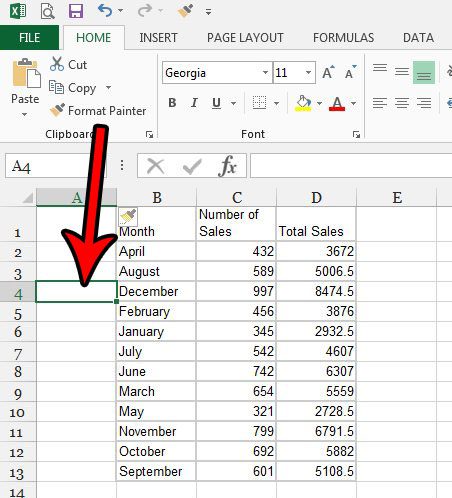
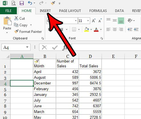
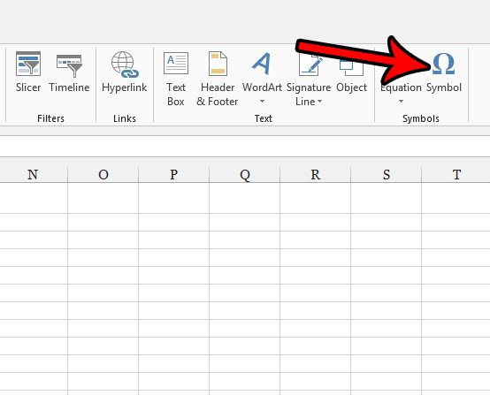
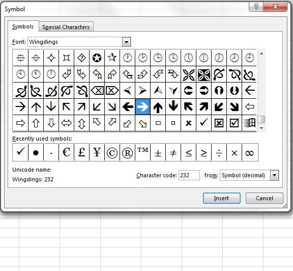
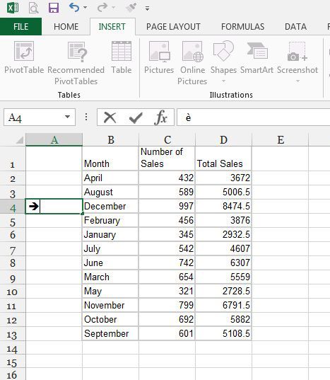
The steps in this article were performed in Microsoft Excel 2013. By completing the steps in this guide you will select a cell in your spreadsheet, then add an arrow to that cell. There are several styles of arrows from which you can select. Step 1: Open your spreadsheet in Excel 2013. Step 2: Select the cell into which you wish to insert the arrow. Step 3: Click the Insert tab at the top of the window. Step 4: Click the Symbol button in the Symbols section at the right side of the ribbon. Step 5: Scroll down the list of symbols until you find the arrow that you want to use, click the desired arrow, then click the Insert button at the bottom of the window. Depending on the arrow you choose, your spreadsheet should them look something like the image below. I use a lot of arrows in the screenshots included on this site, and I typically add them in Photoshop. Find out how to draw arrows in Photoshop if you have that program and a need to perform a similar action.
Additional Sources
After receiving his Bachelor’s and Master’s degrees in Computer Science he spent several years working in IT management for small businesses. However, he now works full time writing content online and creating websites. His main writing topics include iPhones, Microsoft Office, Google Apps, Android, and Photoshop, but he has also written about many other tech topics as well. Read his full bio here.
