One other way to customize the data displayed in your spreadsheet is with the use of filter. By learning how to create a filter in Google Sheets you will unlock a very powerful tool that can provide you with a number of options for displaying subsets of your data. Our tutorial below will show you how to create and set up a filter in Google Sheets and even save that filter so that you can use it again in the future.
See also
How to merge cells in Google SheetsHow to wrap text in Google SheetsHow to alphabetize in Google SheetsHow to subtract in Google SheetsHow to change row height in Google Sheets
How to Use Filters in Google Sheets
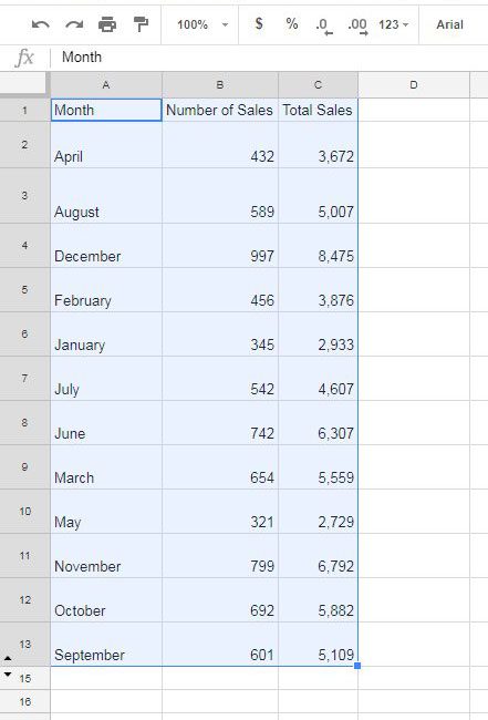
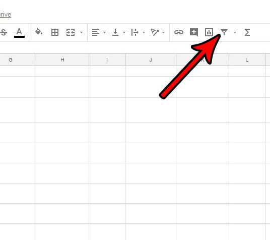
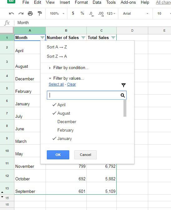
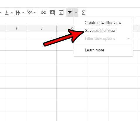
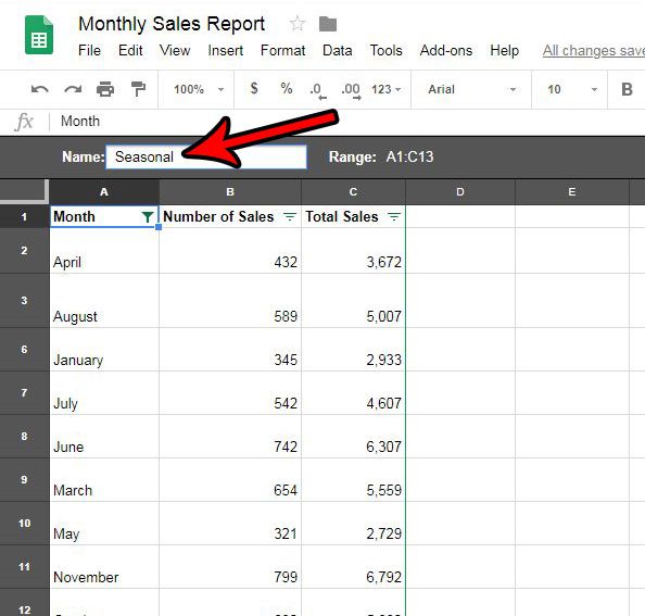
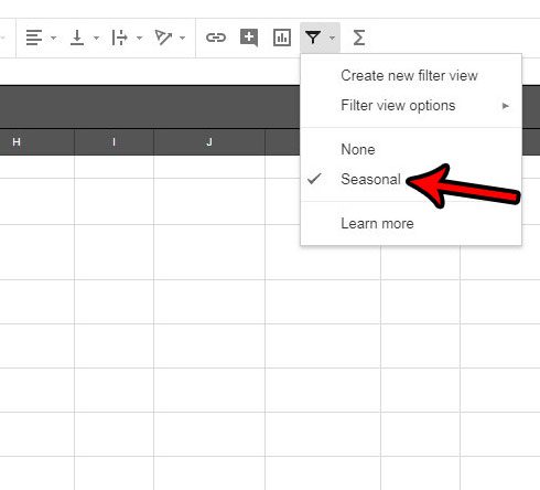
The steps in this article were performed in the desktop version of Google Chrome, but will also work in other desktop Web browsers like Firefox or Edge. This guide assumes that you already have a Google Sheets file with data in it that you would like to filter. We are going to show you how to create the filter, then how to use it to only display some of the data that you have selected. If you like a filter that you have created and want to use it again, you will also have the option of saving that filter. Step 1: Go to your Google Drive at https://drive.google.com and sign into your Google Account if you haven’t already. Step 2: Open the Google Sheets file containing the data that you want to filter. Step 3: Select the data in the spreadsheet that you would like to filter. Step 3: Click the Create a filter button at the right side of the toolbar. Step 4: Click the triangle button at the right side of the column that you want to filter. Step 5: Use the Filter by condition and Filter by values sections of this menu to customize the data that you want to display. You can also use the Sort by options at the top of the menu to change how the data is sorted. Once you’re done, click the OK button at the bottom of the menu. Step 6 (optional): If you like the way that the data is displayed and want to use it again, click the dropdown arrow to the right of the Create a filter button that we clicked in step 3, then choose the Save as filter view option. Step 7 (optional): Type a name for this filter view in the gray bar above the spreadsheet, then press the Enter key on your keyboard to finish. Now when you click the dropdown arrow next to Create a filter again, you will see the filter view that you just saved. You can click that at any time to view the filtered data. Are you looking for a way to combine some of your cells? Find out how to merge cells in Google Sheets if you would like to make some bigger cells without adjusting the sizes of some rows or columns. After receiving his Bachelor’s and Master’s degrees in Computer Science he spent several years working in IT management for small businesses. However, he now works full time writing content online and creating websites. His main writing topics include iPhones, Microsoft Office, Google Apps, Android, and Photoshop, but he has also written about many other tech topics as well. Read his full bio here.
You may opt out at any time. Read our Privacy Policy
