How to Edit Horizontal Axis Labels in Microsoft Excel 2010
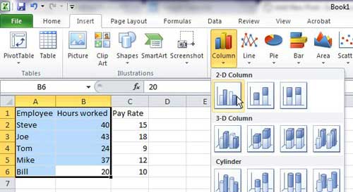
Most of the benefit that comes from using the chart creation tool in Microsoft Excel lies with the one click process of creating the chart, but it is actually a fully-featured utility that you can use to customize the generated chart in a number of different ways. You can modify the horizontal axis labels of your chart, or you can change the unit intervals that Excel chose for the graph based upon the data you selected. To begin, open your Excel spreadsheet that contains the data that you want to graph, or that contains the graph you want to edit. We will go through the entire chart creation process so, if you already have the chart created, you can skip to the part of the tutorial where we are actually changing the horizontal axis labels on the chart. Use your mouse to highlight the data that you want to include in the chart. You can choose to include the column labels for your data if you want to, but Excel will use them in the chart regardless. Click the Insert tab at the top of the window, then click the type of chart that you want to create from the various options in the Charts section of the ribbon.
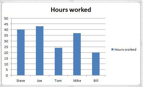
Once your chart has been generated, the horizontal axis labels will be populated based upon the data in the cells that you selected. For example, in the chart image below, the horizontal axis labels are the first names of some fake employees.
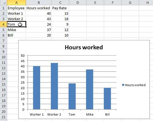
If, for example, I wanted to add some anonymity to the chart, I might choose to relabel these employees with more generic terms, such as “Worker 1”, “Worker 2”, etc. You can do this by changing the values in the cells from which the chart is being populated. If you do not want to change the data in these cells, then you should insert a new column to the right or left of the current column and add the axis labels that you want to use in the new column. My partially modified chart and data are shown in the image below.
Once you experiment with the charts feature of Excel for a little while, you will start to understand exactly how it works. The chart is not storing any extra data or information about your spreadsheet. Everything on the chart is populated from your data so, if you want to make changes to the chart, it must be done from your data. If you want to change other options of the horizontal axis, right-click on one of the axis labels on the chart, then click Format Axis. After receiving his Bachelor’s and Master’s degrees in Computer Science he spent several years working in IT management for small businesses. However, he now works full time writing content online and creating websites. His main writing topics include iPhones, Microsoft Office, Google Apps, Android, and Photoshop, but he has also written about many other tech topics as well. Read his full bio here.
You may opt out at any time. Read our Privacy Policy